Sorry, your browser cannot access this site
This page requires browser support (enable) JavaScript
Learn more >

In cancer research, comparing genomic features between tumor samples and organoid models is crucial for validating model reliability. Circos plots provide an intuitive way to visualize detected mutations across the genome, making them commonly used for representing overall detection results of representative samples. While reading the circlize documentation, I came across an example demonstrating paired samples, which I found suitable for showcasing paired primary samples and organoids. I’ve adapted it to create a plot for displaying paired samples. The code is primarily based on the official documentation’s 9.5 Concatenating two genomes

Preparation

Loading Necessary R Packages

First, we need to load some essential R packages:

1
2
3
4
5
library(circlize)
library(dplyr)
library(stringr)
library(MutationalPatterns)
library(BSgenome.Hsapiens.UCSC.hg38)

Among these, MutationalPatterns is mainly used for loading VCF files to avoid manual processing, while BSgenome.Hsapiens.UCSC.hg38 provides the necessary information for drawing basic chromosomal regions.

Data Preparation

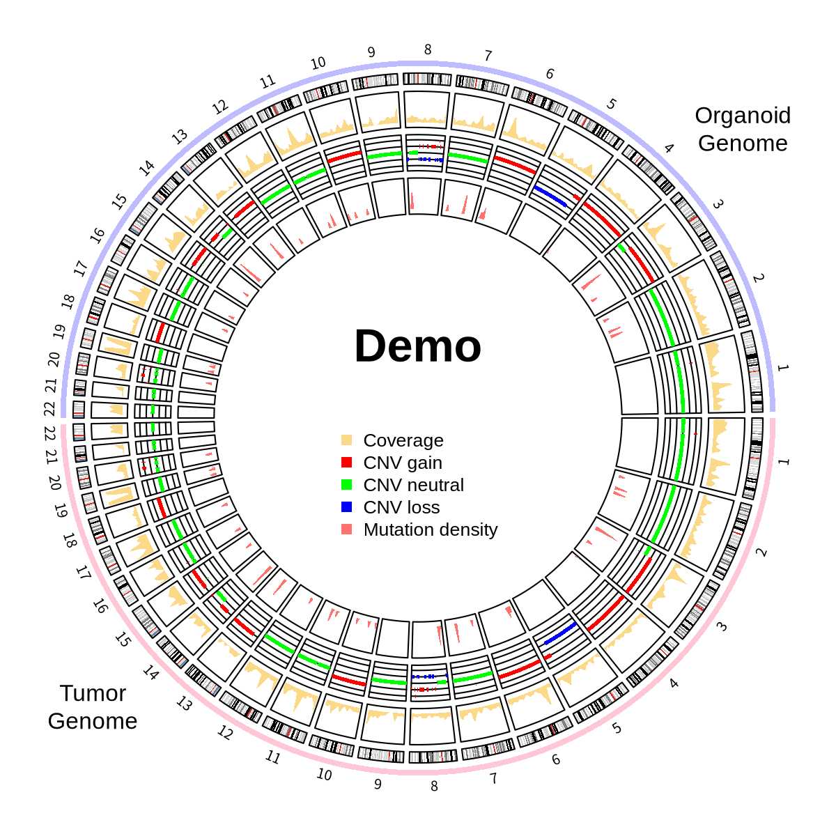
This visualization showcases three types of information:

  • Somatic mutation detection results (VCF files)
  • CNV detection results (from CNVKit)
  • Sequencing coverage data (directly using results from CNV software to avoid duplication)

Building Genomic Framework Data

We first construct a combined framework containing both tumor and organoid genomes:

1
2
3
4
5
6
7
# Remove XY chromosomes and build combined genomic data
tumor_cytoband <- read.cytoband(species = "hg38")$df %>% filter(!(V1 %in% c('chrX', 'chrY')))
organoid_cytoband <- read.cytoband(species = "hg38")$df %>% filter(!(V1 %in% c('chrX', 'chrY')))

tumor_cytoband[ ,1] <- paste0("tumor_", tumor_cytoband[, 1])
organoid_cytoband[ ,1] <- paste0("organoid_", organoid_cytoband[, 1])
cytoband <- rbind(tumor_cytoband, organoid_cytoband)

This creates a data frame named cytoband that contains basic information about the two genomes to be visualized.

Processing Mutation Data

Using the MutationalPatterns package to read VCF files and convert them to a suitable format for plotting:

1
2
3
4
5
6
7
8
9
10
11
12
13
14
15
16
17
18
19
vcfs <- read_vcfs_as_granges(
c(
'tumor.vcf',
'pdo.vcf'
),
c("tumor", "pdo"),
"BSgenome.Hsapiens.UCSC.hg38"
)

mut_data <- rbind(
data.frame(vcfs[[t_sample]]) %>%
mutate(value = 1) %>%
mutate(seqnames = str_c("tumor_", seqnames)) %>%
select(seqnames, start, end, value),
data.frame(vcfs[[o_sample]]) %>%
mutate(value = 1) %>%
mutate(seqnames = str_c("organoid_", seqnames)) %>%
select(seqnames, start, end, value)
)

Processing CNV and Coverage Data

Both CNV and coverage data are obtained from CNVkit:

1
2
3
4
5
6
7
8
9
10
11
12
13
14
15
16
17
18
19
20
21
22
23
24
25
26
27
28
29
30
31
# CNV data
cnv_data <- rbind(
read.table(
"tumor.cnvkit.call.cns",
sep="\t", header = F,
col.names = c("chromosome", "start", "end", "cn")
) %>%
mutate(value = cn) %>%
mutate(chromosome = str_c("tumor_", chromosome)) %>%
select(chromosome, start, end, value),
read.table(
"pdo.cnvkit.call.cns",
sep="\t", header = F,
col.names = c("chromosome", "start", "end", "cn")
) %>%
mutate(value = cn) %>%
mutate(chromosome = str_c("organoid_", chromosome)) %>%
select(chromosome, start, end, value)
) %>% mutate(value = pmin(value, 4)) # Limit CNV values to maximum of 4

# Coverage data
cov_data <- rbind(
read.table("tumor.cnvkit.cov.cnn", sep="\t", header = T) %>%
mutate(value = log2) %>%
mutate(chromosome = str_c("tumor_", chromosome)) %>%
select(chromosome, start, end, value),
read.table("pdo.cnvkit.cov.cnn", sep="\t", header = T) %>%
mutate(value = log2) %>%
mutate(chromosome = str_c("organoid_", chromosome)) %>%
select(chromosome, start, end, value)
)

Drawing the Circos Plot

Setting Colors and Initialization

1
2
3
4
5
6
7
8
9
10
11
12
13
14
15
16
17
18
19
20
21
22
23
# Color settings
red <- "#FFC6D6"
blue <- "#bebcff"
green <- "#9CCF83"
orange <- "#fbd988ff"
purpule <- "#ff726dff"
black <- "#000000"

# Set image size
png(filename = "demo.circos.png", width = 1200, height = 1200, res = 200)

# Build basic circos framework
chromosome.index = c(
paste0("tumor_chr", c(1:22)),
rev(paste0("organoid_chr", c(1:22)))
)

circos.par(gap.after = c(rep(1, 22), rep(1, 22)))
circos.initializeWithIdeogram(
cytoband,
plotType = NULL,
chromosome.index = chromosome.index
)

Adding Chromosome Tracks

1
2
3
4
5
6
7
8
9
10
11
12
13
14
# Set chromosome track
circos.track(
ylim = c(0, 1),
panel.fun = function(x, y) {
circos.text(CELL_META$xcenter, CELL_META$ylim[2] + mm_y(2),
gsub(".*chr", "", CELL_META$sector.index), cex = 0.6, niceFacing = TRUE)
},
track.height = mm_h(1),
cell.padding = c(0, 0, 0, 0),
bg.border = NA
)
highlight.chromosome(paste0("tumor_chr", c(1:22)), col = red, track.index = 1)
highlight.chromosome(paste0("organoid_chr", c(1:22)), col = blue, track.index = 1)
circos.genomicIdeogram(cytoband)

Adding Coverage, CNV, and Mutation Density Tracks

1
2
3
4
5
6
7
8
9
10
11
12
13
14
15
16
17
18
19
20
21
22
23
# Sequencing coverage
circos.genomicDensity(cov_data, col=orange, track.height = 0.1, window.size = 1e7)

# CNV track
circos.genomicTrackPlotRegion(
cnv_data,
ylim = c(0, 4),
panel.fun = function(region, value, ...) {
cell.xlim = get.cell.meta.data("cell.xlim")
for(h in c(0, 1, 2, 3, 4)) {
circos.lines(cell.xlim, c(h, h), col = black)
}
col = ifelse(value[[1]] > 2, "red",
ifelse(value[[1]] == 2, "green", "blue")
)
i = getI(...)
circos.genomicRect(region, value, col = col, ytop = value + 0.3, ybottom = value - 0.3 , border = NA)
},
track.height = 0.1
)

# Mutation density
circos.genomicDensity(mut_data, col=purpule, track.height = 0.1, window.size = 1e7)

Adding Text and Legend

1
2
3
4
5
6
7
8
9
10
11
12
13
14
15
16
17
18
19
20
21
# Set center text
text(0, 0.2, "Demo", cex = 2, font = 2)
# Set corner text
text(-0.9, -0.8, "Tumor\nGenome")
text(0.9, 0.8, "Organoid\nGenome")

# Set legend below center text
legend(
x = 0,
y = 0,
legend = c("Coverage", "CNV gain", "CNV neutral", "CNV loss", "Mutation density"),
col = c(orange, "red", "green", "blue", purpule),
pch = 15,
pt.cex = 1,
cex = 0.8,
bty = "n",
xjust = 0.5,
)

circos.clear()
dev.off()

Complete Code

1
2
3
4
5
6
7
8
9
10
11
12
13
14
15
16
17
18
19
20
21
22
23
24
25
26
27
28
29
30
31
32
33
34
35
36
37
38
39
40
41
42
43
44
45
46
47
48
49
50
51
52
53
54
55
56
57
58
59
60
61
62
63
64
65
66
67
68
69
70
71
72
73
74
75
76
77
78
79
80
81
82
83
84
85
86
87
88
89
90
91
92
93
94
95
96
97
98
99
100
101
102
103
104
105
106
107
108
109
110
111
112
113
114
115
116
117
118
119
120
121
122
123
124
125
126
127
128
129
130
131
132
133
134
135
136
137
138
139
140
141
142
143
144
library(circlize)
library(dplyr)
library(stringr)
library(MutationalPatterns)
library(BSgenome.Hsapiens.UCSC.hg38)

tumor_cytoband <- read.cytoband(species = "hg38")$df %>% filter(!(V1 %in% c('chrX', 'chrY')))
organoid_cytoband <- read.cytoband(species = "hg38")$df %>% filter(!(V1 %in% c('chrX', 'chrY')))

tumor_cytoband[ ,1] <- paste0("tumor_", tumor_cytoband[, 1])
organoid_cytoband[ ,1] <- paste0("organoid_", organoid_cytoband[, 1])
cytoband <- rbind(tumor_cytoband, organoid_cytoband)

t_sample <- "tumor"
o_sample <- "pdo"

vcfs <- read_vcfs_as_granges(
c(
'tumor.vcf',
'pdo.vcf'
),
c(t_sample, o_sample),
"BSgenome.Hsapiens.UCSC.hg38"
)

mut_data <- rbind(
data.frame(vcfs[[t_sample]]) %>%
mutate(value = 1) %>%
mutate(seqnames = str_c("tumor_", seqnames)) %>%
select(seqnames, start, end, value),
data.frame(vcfs[[o_sample]]) %>%
mutate(value = 1) %>%
mutate(seqnames = str_c("organoid_", seqnames)) %>%
select(seqnames, start, end, value)
)


cnv_data <- rbind(
read.table(
"tumor.cnvkit.call.cns",
sep="\t", header = T
) %>%
mutate(value = cn) %>%
mutate(chromosome = str_c("tumor_", chromosome)) %>%
select(chromosome, start, end, value),
read.table(
"pdo.cnvkit.call.cns",
sep="\t", header = T
) %>%
mutate(value = cn) %>%
mutate(chromosome = str_c("organoid_", chromosome)) %>%
select(chromosome, start, end, value)
) %>% mutate(value = pmin(value, 4))


cov_data <- rbind(
read.table("tumor.cnvkit.cov.cnn", sep="\t", header = T) %>%
mutate(value = log2) %>%
mutate(chromosome = str_c("tumor_", chromosome)) %>%
select(chromosome, start, end, value),
read.table("pdo.cnvkit.cov.cnn", sep="\t", header = T) %>%
mutate(value = log2) %>%
mutate(chromosome = str_c("organoid_", chromosome)) %>%
select(chromosome, start, end, value)
)


########################################### Plotting ###########################################

red <- "#FFC6D6"
blue <- "#bebcff"
green <- "#9CCF83"
orange <- "#fbd988ff"
purpule <- "#ff726dff"
black <- "#000000"

png(filename = "demo.circos.png", width = 1200, height = 1200, res = 200)

chromosome.index = c(
paste0("tumor_chr", c(1:22)),
rev(paste0("organoid_chr", c(1:22)))
)

circos.par(gap.after = c(rep(1, 22), rep(1, 22))) # Set gaps?
circos.initializeWithIdeogram(
cytoband,
plotType = NULL,
chromosome.index = chromosome.index
)

circos.track(
ylim = c(0, 1),
panel.fun = function(x, y) {
circos.text(CELL_META$xcenter, CELL_META$ylim[2] + mm_y(2),
gsub(".*chr", "", CELL_META$sector.index), cex = 0.6, niceFacing = TRUE)
},
track.height = mm_h(1),
cell.padding = c(0, 0, 0, 0),
bg.border = NA
)
highlight.chromosome(paste0("tumor_chr", c(1:22)), col = red, track.index = 1)
highlight.chromosome(paste0("organoid_chr", c(1:22)), col = blue, track.index = 1)
circos.genomicIdeogram(cytoband)

circos.genomicDensity(cov_data, col=orange, track.height = 0.1, window.size = 1e7)

circos.genomicTrackPlotRegion(
cnv_data,
ylim = c(0, 4),
panel.fun = function(region, value, ...) {
cell.xlim = get.cell.meta.data("cell.xlim")
for(h in c(0, 1, 2, 3, 4)) {
circos.lines(cell.xlim, c(h, h), col = black)
}
col = ifelse(value[[1]] > 2, "red",
ifelse(value[[1]] == 2, "green", "blue")
)
i = getI(...)
circos.genomicRect(region, value, col = col, ytop = value + 0.3, ybottom = value - 0.3 , border = NA)
},
track.height = 0.1
)

circos.genomicDensity(mut_data, col=purpule, track.height = 0.1, window.size = 1e7)

text(0, 0.2, "Demo", cex = 2, font = 2)
text(-0.9, -0.8, "Tumor\nGenome")
text(0.9, 0.8, "Organoid\nGenome")

legend(
x = 0,
y = 0,
legend = c("Coverage", "CNV gain", "CNV neutral", "CNV loss", "Mutation density"),
col = c(orange, "red", "green", "blue", purpule),
pch = 15,
pt.cex = 1,
cex = 0.8,
bty = "n",
xjust = 0.5,
)

circos.clear()

dev.off()

Final Result

This uses data generated from one sample to create both the upper and lower circles, so the detection results appear identical on both sides. In reality, if paired results were this consistent, it would be quite remarkable.

circos_demo

Comments

Please leave your comments here